Introduction

In this note, we prove the following theorem, which is a major step toward a proof of the PCP theorem.

Recall that in the optimization problem \({2\text{-CSP}_W}\), we are given a list of arity-\(2\) constraints between variables over an alphabet of size \(W\) and the goal is to find an assignment to the variables that satisfies as many of the constraints as possible.

A \({2\text{-CSP}_W}\) instance \(\varphi\) is \(d\)-regular if every variable of \(\varphi\) appears in exactly \(d\) of the constraints of \(\varphi\). It turns out that there is an efficient reduction to transform general instances of \({2\text{-CSP}_W}\) to \(d\)-regular ones without significantly affecting the optimal value of the instance.

Theorem (gap amplification). For all \(d,t,W\in \bbN\), there exists a polynomial-time linear-blowup function \(f\) that maps every \(d\)-regular \({2\text{-CSP}_W}\) instance \(\varphi\) to a \({2\text{-CSP}_W'}\) instance \(\varphi'=f(\varphi)\),

• YES: if \(\opt(\varphi)=1\), then \(\opt(\varphi')=1\)
• NO: if \(\opt(\varphi)<1-\e\) for some \(\e < 1/(t d)\), then \(\opt(\varphi')<1-\e'\) for \(\e'=t \e / \poly(W,d)\)
• Efficiency: \(\lvert W' \rvert \le \lvert W \rvert^{d^t}\) and \(\lvert \varphi' \rvert\le \lvert \varphi' \rvert\cdot O(d^t)\)

Interlude: Spectral graph expansion

A graph \(G\) is \(d\)-regular if every vertex of \(G\) is an endpoint of exactly \(d\) edges of \(G\).

Let \(G\) be a \(d\)-regular graph \(G\) with \(n\) vertices. Its normalized adjacency matrix \(A_G\) is an \(n\)-by-\(n\) matrix indexed by the vertices of \(G\) such that \[ (A_G)_{u,v} = \begin{cases} 1/d & \text{if $(u,v)\in E(G)$}\,,\\ 0 & \text{otherwise.} \end{cases} \] We extend this definition to graphs with parallel edges and self-loops: We set \((A_G)_{u,v}\) to the fraction of \(u\)’s edges that are incident to \(v\).

The following observation shows how \(A_G\) acts on real-valued vectors indexed by vertices of \(G\).

Observation (averaging over neighbors). For every vector \(x\in \R^{V(G)}\) and every vertex \(u\in V(G)\), \[ (A_G x)_u = \text{average $x$-value of the neighbors of $u$}\,.\notag \]

Since the matrix \(A_G\) is symmetric and real-valued, its eigenvalues \(\lambda_1,\ldots,\lambda_n\) are real.

Claim. All eigenvalues of \(A_G\) are contained in the interval \([-1,1]\).

Proof. We use the following general bound on the largest eigenvalue in absolute value of a symmetric matrix, \[ \max_{i\in [n]} \lvert \lambda_i \rvert \le \max_{u\in V(G)} \sum_{v\in V(G)} \lvert (A_G)_{u,v} \rvert = 1\,. \]

Claim. The vector \(\mathbf{1}=(1,\ldots,1)^T\) is an eigenvector of \(A_G\) with value \(1\).

Proof. The averaging-over-neighbors observation shows that \(A\mathbf 1= \mathbf 1\).

The previous two claims show that we can order the eigenvalues of \(A_G\) such that \[ 1=\lambda_1 \ge \lvert \lambda_2 \rvert \ge \cdots \ge \lvert \lambda_n \rvert\,. \]

Definition (Spectral expansion). For every regular graph, we define its spectral expansion \(\lambda(G)=\lambda_2\) as the second largest eigenvalue in absolute value of \(G\)’s normalized adjacency matrix.

The following lemma gives a combinatorial characterization of the condition \(\lambda(G)<1\). Its proof is an exercise.

Lemma. A graph \(G\) is connected and non-bipartite if and only if \(\lambda(G)<1\).

It turns out that the spectral expansion parameter \(\lambda\) is a surprisingly useful way to quantify the “connectedness” and “non-bipartiteness” of a graph. Graphs with spectral expansion bounded away from \(1\), say \(\lambda<0.9\), behave in many ways similar to random graphs. We refer to such graphs as expander graphs.

Definition (Expander graphs). A collection \(\{G_n\mid n\in \bbN\}\) of graphs is called a family of expander graphs if there exists a constant \(\lambda<1\) such that every graph \(G_n\) in the family satisfies \(\lambda(G_n)\le \lambda\).

For every \(d\ge 3\), there exist families of \(d\)-regular expander graphs and they can be computed in polynomial time. (In fact, a random \(d\)-regular graph is an expander with high probability.)

The following property of expander graphs is useful for the analysis of our gap amplification construction. Its proof is an exercise.

Lemma (Expander mixing lemma). For every regular graph \(G\) and every set \(S\subseteq V(G)\), \[ \Pr_{uv\in E(G)}\biggl\{ u\in S \land v\in S\biggr\} \le \Pr_{u\in V(G)}\bigl\{u\in S\bigr\} \cdot \biggl(\Pr_{v\in V(G)}\bigl\{v\in S\bigr\} + \lambda (G)\biggr) \,. \]

Note that the upper bound \(\Pr_{uv\in E(G)}\{ u\in S \land v\in S\}\le \Pr_{u\in V(G)}\{u\in S\}\) holds for every graph \(G\) and every set \(S\subseteq V(G)\). The expander mixing lemma implies that this upper bound is far from tight whenever the spectral expansion of \(G\) is bounded away from \(1\) and the set \(S\) excludes a constant fraction of the vertices of \(G\).

If we choose \(S\) as a random set of size \(k\) in a regular graph \(G\) with \(n\) vertices, then \[ \E_{\substack{S\subseteq V(G)\\ \lvert S \rvert = k}} \Pr_{uv\in E(G)}\biggl\{ u\in S \land v\in S\biggr\} \approx \frac{k}{n} \cdot \frac{k}{n} \,. \] The expander mixing lemma implies that every set \(S\subseteq V(G)\) of size \(k\) satisfies \(\Pr_{uv\in E(G)}\biggl\{ u\in S \land v\in S\biggr\} \approx \frac{k}{n} \cdot \frac{k}{n}\) if \(\lambda(G)\ll \frac{k}{n}\).

Definition (path power). For a graph \(G\), its \(t\)-fold path power \(G^t\) has the same set of vertices \(V(G^t)=V(G)\) as \(G\) and for every \(t\)-step walk \(u_1,\ldots,u_t\) in \(G\), the graph \(G^t\) contains an edge between the walk endpoints \(u_1\) and \(u_t\).

If \(G\) is \(d\)-regular, then its power \(G^t\) is \(d^t\) regular. (The graph \(G^t\) may have parallel edges and self-loops.) Furthermore, the normalized adjacency matrix of \(G\) and \(G^t\) satisfy the relation, \[ A_{G^t} = (A_G)^t\,. \] Since the eigenvalues of the power of a matrix are the powers of its eigenvalues, the spectral expansion of \(G^t\) is the \(t\)-th power of the spectral expansion of \(G\).

Lemma (spectral expansion of path power). For every graph \(G\) and every \(t\in \bbN\), the \(t\)-fold path power \(G^t\) has spectral expansion \(\lambda(G^t) = \lambda(G)^t\).

This lemma shows that the path power operation improves spectral expansion. This fact underlies some of the constructions of expander graphs.

Gap amplification construction

Let \(\varphi\) be a \(d\)-regular \({2\text{-CSP}_W}\) instance with variables \(x_1,\ldots,x_n\) over alphabet \([W]\). Let \(G\) be the constraint graph of \(\varphi\), i.e., the \(d\)-regular graph on \([n]\) that has an edge between vertices \(u\in [n]\) and \(v\in [n]\) for every constraint between variables \(x_u\) and \(x_v\) in \(\varphi\). For an edge \(e\in E(G)\) between \(u\) and \(v\), let \(\varphi_e\from [W]\times [W] \to \{0,1\}\) be the corresponding constraint in \(\varphi\). Then, the objective value of an assignment \(x\in [W]^n\) for \(\varphi\), denoted \(\varphi(x)\), satisfies \[ \varphi(x) = \Pr_{e=(u,v) \in E(G)}\biggl\{ \varphi_e (x_u, x_v) = 1 \biggr\}\,. \]

For every vertex \(u\in V(G)\), let \(N_t(u)\subseteq V(G)\) denote the \(t\)-step neighborhood of \(u\) in \(G\), i.e., all vertices that can be reached from \(u\) by a path of length at most \(t\).

Construction of \({2\text{-CSP}_W'}\) instance \(\varphi^t\).

• variables: \(y_1,\ldots,y_n\)
• alphabet: size \(W' = W^{d^t}\); for variable \(y_u\), we identify alphabet with an assignments to the \(t\)-step neighborhood \(N_t(u)\) so that \(y_u\) takes values in \([W]^{N(t)}\); we refer to \((y_u)_v\) as the “opinion” of \(u\) about \(v\).
• constraints: for every edge \((u,v)\in E(G^t)\), we have the following constraint \(\varphi_{u,v}\from W^{N_t(u)} \times W^{N_t(v)} \to \{0,1\}\), \[ \varphi^t_{u,v} (y_u, y_v) = 1 \Leftrightarrow \left \{\begin{aligned} & \text{the assignments $y_u$ and $y_v$ agree on $N_t(u)\cap N_t(v)$ and}\\ & \text{satisfy all constraints of $\varphi$ between variables in $N_t(u)\cup N_t(v)$} \end{aligned} \right \} \]

This construction satisfies the desired YES property (for the gap amplification theorem): If \(\opt(\varphi)=1\), then \(\opt(\varphi^t)=1\). Concretely, if \(x_1,\ldots,x_n\) is an assignment for \(\varphi\) that satisfies all constraints, then the following assignment \(y_1,\ldots,y_n\) satisfies all constraints of \(\varphi^t\), \[ \forall u,v\in [n].\quad (y_u)_v = x_v\,. \] The construction of \(\varphi^t\) also satisfies the desired efficiency property: The number of constraints in \(\varphi^t\) is at most \(d^t\) factor larger than the number of constraints in \(\varphi\). Therefore, \(\lvert \varphi^t \rvert \le \lvert \varphi \rvert \cdot O(d^t)\).

Analysis against consistent assignments

In order to finish the proof of the gap amplification theorem it remains to establish the NO property of the construction of \(\varphi^t\).

Let \(\varphi\) be a \(d\)-regular instance of \({2\text{-CSP}_W}\). Suppose that \(\opt(\varphi)<1-\varepsilon\) for some \(\varepsilon < 1/(d t)\). We are to show that \(\opt(\varphi^t) < 1- t \e / \poly(d,W)\).

As a first step toward this goal, we show that all “consistent assignment” for \(\varphi^t\) indeed achieve objective value at most \(1- t \e / \poly(d)\) as long as the constraint graph \(G\) of \(\varphi\) has graph expansion \(\lambda(G)\) bounded away from \(1\). The assumption that the constraint graph has \(\lambda(G)\) bounded away from \(1\) is without loss of generality because we can ensure this property by adding constraints to \(\varphi\) that are always satisfied and have an \(d\)-regular expander as constraint graph.

Definition. We say that an assignment \(y_1,\ldots,y_n\) is consistent if there exists an assignment \(x_1,\ldots,x_n\) such that \((y_u)_v=x_v\) for all \(u,v\in [n]\).

Lemma. Suppose the constraint graph \(G\) of \(\varphi\) satisfies \(\lambda(G)<0.9\). Then, every consistent assignment \(y\) has objective value at most \(1-t \varepsilon / 100d\) for \(\varphi^t\).

Modified construction (easier analysis)

So far we know that the construction of \(\varphi^t\) satisfies the desired NO property if we restrict ourselves to consistent assignments. We modify the construction slightly in order to simplify the analysis against all assignments.

The modified construction of \(\varphi^t\) is the same as before except that we assign different weights to the new constraints \(\varphi^t_{u,v}\). The modified construction has a parameter \(\delta >0\). (We can choose \(\delta = 1/(4W)\).)

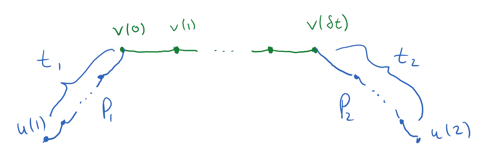
Weights of constraints in modified construction. The weight of the constraint \(\varphi^t_{u(1),u(2)}\) in \(\varphi^t\) is equal to the probability of \(u(1)\) and \(u(2)\) being generated by the following randomized algorithm:

• choose a random path \(v(1),\ldots,v(t_0)\) of length \(\delta t\) in the constraint graph \(G\) of \(\varphi\)
• choose integers \(t_1,t_2\) uniformly at random from interval \([t/2,t]\)
• choose a random path \(P_1\) from \(v(1)\) of length \(t_1\) and a random path \(P_2\) from \(v( t_0)\) of length \(t_2\)
• let \(u(1)\) be the endpoint of \(P_1\) and \(u(2)\) be the endpoint of \(P_2\)

Analysis against all assignments

Let \(y\) be an arbitrary assignment for \(\varphi^t\) (not necessarily consistent). We are to upper bound the objective value of \(y\).

Our strategy is to construct an assignment \(x\) for \(\varphi\) from the assignment \(y\) for \(\varphi^t\). We then use the constraints violated by \(x\) in order to bound the objective value of \(y\) for \(\varphi^t\).

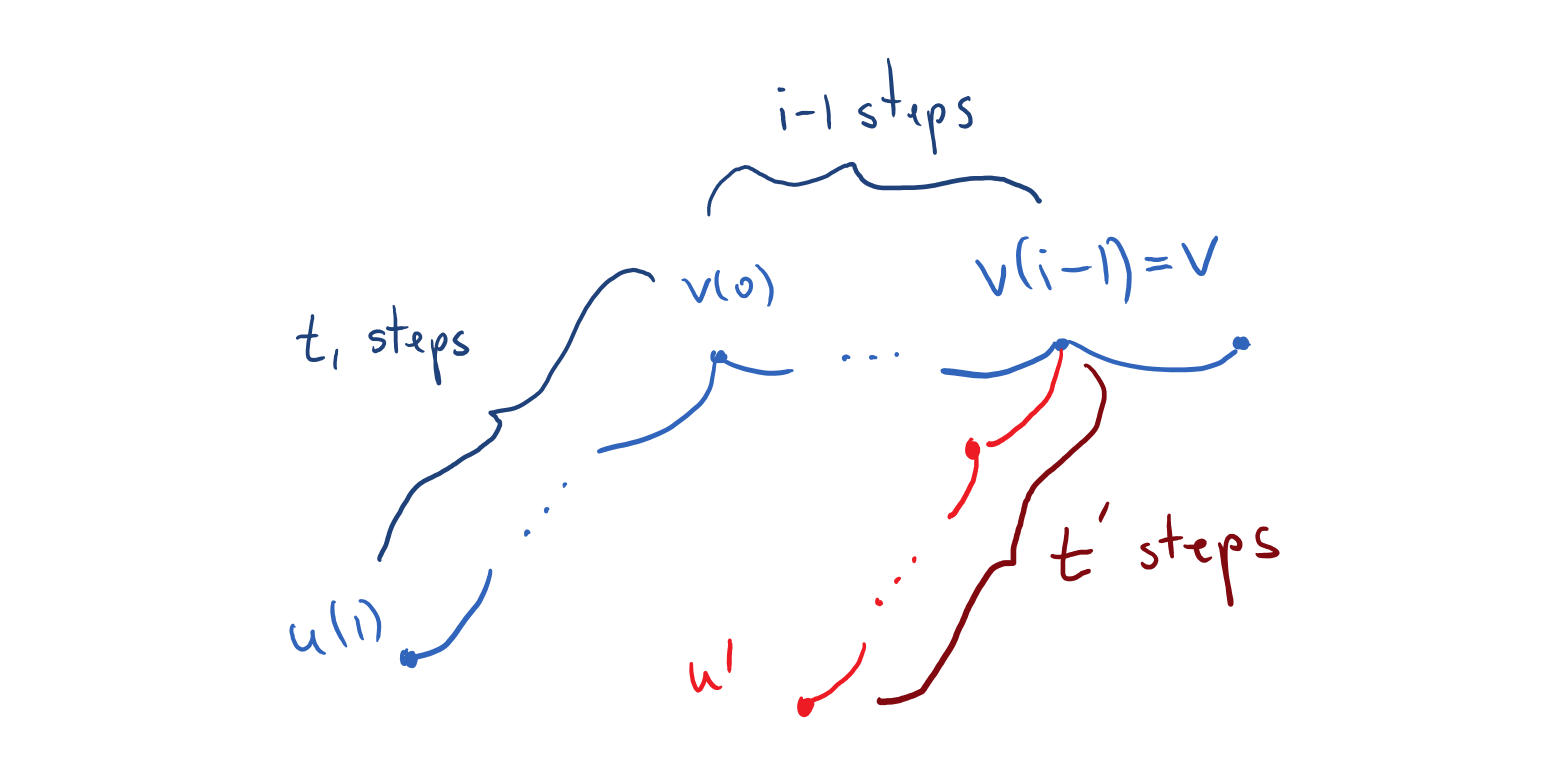
Plurality assignment obtained from \(y\). Let \(x\) be the assignment for \(\varphi\) such that for every vertex \(v\), we choose \(x_v\) as the most likely output of the following randomized algorithm:

• choose an integer \(t'\) uniformly at random from the interval \([t/2,t]\)
• choose a random path \(P'\) from \(v\) of length \(t'\)
• let \(u'\) be the endpoint of \(P'\)
• output \((y_{u'})_v\in [W]\), that is, the opinion of \(u'\) about \(v\)

Note that if \(y\) is consistent with an assignment \(x\) for \(\varphi\), then \(x\) is also the plurality assignment constructed above.

Let \(\eta>0\) be the fraction of constraints not satisfied by the plurality assignment \(x\). For every \(i\in [\delta t]\), let \(X_i\) be the indicator random variable such that \(X_i=1\) if and only if all of the following conditions are satisfied

• the constraint between \(v(i-1)\) and \(v(i)\) in \(\varphi\) is not satisfied by the plurality assignment \(x\)
• the opinion \((y_{u(1)})_{v(i-1)}\) of \(u(1)\) about \(v(i-1)\) differs from the plurality assignment \(x_{v(i-1)}\)
• the opinion \((y_{u(2)})_{v(i)}\) of \(u(2)\) about \(v(i)\) differs from the plurality assignment \(x_{v(i)}\)

Note that if \(X_i=1\), then the assignment \(y\) does not satisfy the constraint between \(u(1)\) and \(u(2)\) in \(\varphi^t\). Let \(X=X_{1} + \cdots + X_{\delta t}\). As before, we can lower bound the fraction of constraints not satisfied by \(y\) in terms of the first two moments of \(X\), \[ \Pr\biggl\{ \varphi^t_{u(1),u(2)}\bigl(y_{u(1)},y_{u(2)}\bigr) =0 \biggr\} \ge \Pr\biggl\{ X>0 \biggr\} \ge (\E X)^2 / \E X^2\,. \label{eq:moment-lower-bound} \]

It remains to estimate the first two moments of \(X\). It turns out that in order to show the bound \(\E X^2 \le 30 d t \eta\) essentially the same proof works as before. However the lower bound on \(\E X\) requires new ideas. In particular, we will use basic properties of the statistical distance between random variables (related to the total variation distance of probability distributions).

Definition. For (finitely-supported) random variables \(A\) and \(B\), let \(\Delta(A,B)\) be their statistical distance, \[ \Delta\bigl(A,B\bigr) = \sum_{\omega \in \mathrm{support}(A) \cup \mathrm{support}(B)} \bigl\lvert \Pr\{ A = \omega\} - \Pr\{ B = \omega\} \bigr\rvert/2 \]

Claim 3. For every \(i\in [t]\), we have \[ \begin{gathered} \Pr \biggl\{ \bigl(y_{u(1)}\bigr)_{v(i-1)} = x_{v(i-1)} \land \bigl(y_{u(2)}\bigr)_{v(i)} = x_{v(i)} \biggm \vert v(i-1), v(i) \biggr\} \ge \left (\frac 1 W - 2\delta\right)^2\\ \end{gathered} \]

Proof. Since \(u(1)\) and \(u(2)\) are statistically independent conditioned on \(\{v(i-1), v(i)\}\), it is enough to show that each of the events \(\{(y_{u(1)})_{v(i-1)} = x_{v(i-1)}\}\) and \(\{(y_{u(2)})_{v(i)} = x_{v(i)}\}\) have probability at least \(1/W - 2 \delta\) conditioned on \(\{v(i-1), v(i)\}\). By symmetry between \(u(1)\) and \(u(2)\), it remains to show that \[ \Pr \biggl\{ \bigl(y_{u(1)}\bigr)_{v(i-1)} = x_{v(i-1)} \biggm \vert v(i-1), v(i) \biggr\} \ge \frac 1 W - 2\delta\,. \label{eq:almost-plurality-prob} \]

Let \((t',P',u')\) be the random variables as defined in the construction of the plurality assignment for \(x_{v}\) with \(v=v(i-1)\). Since \(x_{v(i-1)}\) is the most likely value for \((y_{u'})_{v}\) and there are only \(W\) possible outcomes, we have \[ \Pr \biggl\{ \bigl(y_{u'}\bigr)_{v(i-1)} = x_{v(i-1)} \biggm \vert v(i-1) \biggr\} \ge \frac 1 W \,. \label{eq:plurality-prob} \]

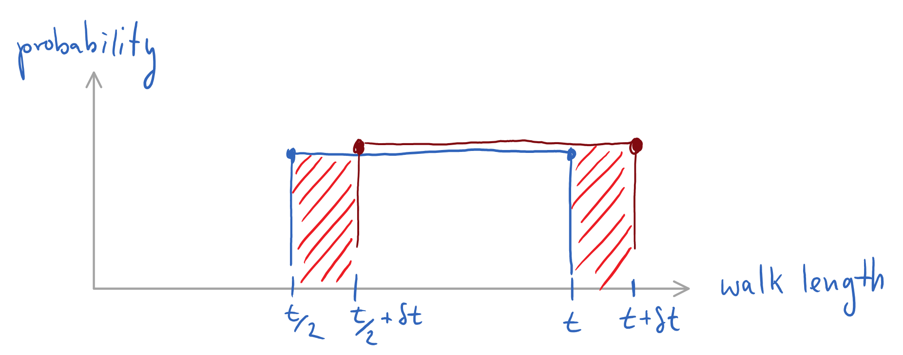
We connect the bound \(\eqref{eq:plurality-prob}\) to the target \(\eqref{eq:almost-plurality-prob}\) by estimating the statistical distance between \(\bigl(y_{u'}\bigr)_{v(i-1)}\) and \(\bigl(y_{u(1)}\bigr)_{v(i-1)}\) conditioned on \(v(i-1)\), \[ \begin{aligned} \Delta\biggl(\bigl\{(y_{u(1)})_{v(i-1)} \bigm \vert v(i-1)\bigr\}, \bigl\{(y_{u'})_{v(i-1)} \bigm \vert v(i-1)\bigr\} \biggr) & \le \Delta\biggl(\bigl\{u(1)\bigm \vert v(i-1)\bigr\}, \bigl\{u' \bigm \vert v(i-1)\bigr\} \biggr)\\ & \le \Delta\biggl(t_1 + i-1, t' \biggr)\\ & \le \frac{{(i-1)}}{t/2}\,. \end{aligned} \] It is instructive to verify the above computation first for the case \(i=1\). Here the statistical distance is indeed \(0\) because both \(u(1)\) and \(u'\) are generated in the same way—by a random walk from \(v(0)\) whose length is uniformly distributed in \([t/2,t]\). For larger values of \(i\), the statistical distance arises because \(u(1)\) and \(u'\) are generated by random walks with differently distributed lengths. The length of the random walk for \(u'\) is still uniformly distributed in \([t/2,t]\). However, the length of the random walk for \(u(1)\) (when viewed from \(v(i-1)\)) is uniformly distributed between \(i-1+t/2\) and \(i-1+t\). The statistical distance between these two distributions for random walk lengths is \((i-1)/(t/2)\). Formally, the reasoning among uses the data processing inequality for statistical distance (see for example these lecture notes as a reference).

We conclude the desired bound \(\eqref{eq:almost-plurality-prob}\) by \[ \begin{aligned} & \Pr \biggl\{ \bigl(y_{u(1)}\bigr)_{v(i-1)} = x_{v(i-1)} \biggm \vert v(i-1), v(i) \biggr\} \\ & \ge \Pr \biggl\{ \bigl(y_{u'}\bigr)_{v(i-1)} = x_{v(i-1)} \biggm \vert v(i-1) \biggr\} \\ & \quad - \Delta\biggl(\bigl\{(y_{u(1)})_{v(i-1)} \bigm \vert v(i-1)\bigr\}, \bigl\{(y_{u'})_{v(i-1)} \bigm \vert v(i-1)\bigr\} \biggr) \\ & \ge 1/W - (i-1)/(t/2) \ge 1/W - 2\delta\,.\qed \end{aligned} \]

The previous claim allows us to show the desired lower bound on \(\E X\).

Claim 4. \(\E X \ge \delta t \eta \cdot \left(\frac 1 W - 2\delta\right)^2\). In particular, if we choose \(\delta = 1/(4W)\), then \(\E X \ge t \eta / (16 W^2)\).

Proof. By linearity of expectation, \(\E X = \sum_i \E X_i\). Thus, it suffices to show that every \(i\) satisfies \(\E X_i\ge \eta / (100 W^2)\). Indeed, by the definition of \(X_i\), \[ \begin{aligned} \E X_i & = \Pr\biggl\{ \varphi_{v(i-1),v(i)}(x_{v(i-1), x_{v(i)}})=0 \biggr\} \\ & \quad \cdot \Pr \biggl\{ \bigl(y_{u(1)}\bigr)_{v(i-1)} = x_{v(i-1)} \land \bigl(y_{u(2)}\bigr)_{v(i)} = x_{v(i)} \biggm \vert v(i-1), v(i) \biggr\} \\ & \ge \Pr\biggl\{ \varphi_{v(i-1),v(i)}(x_{v(i-1), x_{v(i)}})=0 \biggr\} \cdot \left(\frac 1 W - 2\delta\right)^2\\ &= \eta \cdot \left(\frac 1 W - 2\delta\right)^2 \end{aligned} \] The first inequality is by Claim 3. The last step uses that \(\eta\) is the fraction of constraints not satisfied by the plurality assignment \(x\) in \(\varphi\).

The same proof as for Claim 2 bounds the second moment of \(X\) (again under the mild assumption that \(\lambda(G)<0.9\)).

Claim 5. \(\E X^2\le 30 d t \eta\).

At this point, we have all components of the proof of the gap amplification theorem.